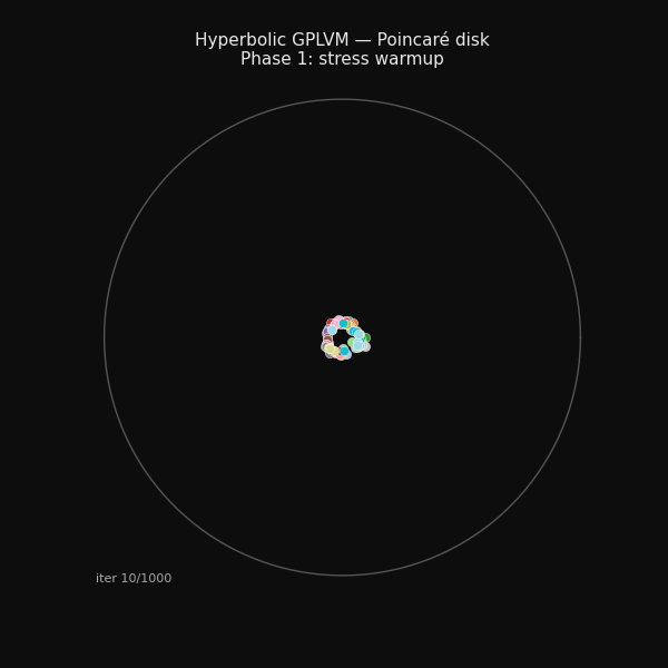
94 hand-grasp recordings arranging themselves on the Poincaré disk during training.
Phase 1: stress warmup
Phase 2: joint GP + stress
A from-scratch implementation of the core model in Jaquier et al., ICML 2024 — learning a continuous latent space that respects a discrete motion taxonomy, using the geometry of hyperbolic space.
94 hand-grasp recordings arranging themselves on the Poincaré disk during training.
Phase 1: stress warmup
Phase 2: joint GP + stress
Human knowledge about motion is hierarchical. Hand grasps form a taxonomy tree — Tripod and Lateral are precision grasps; Wrap is a power grasp. Some grasps are cousins, some are distant relatives. That structure is discrete.
Robot joint angles are continuous — 24 floating-point numbers per recording. The question is: can we learn a 2D map of joint-angle recordings where taxonomically similar grasps land close together?
The answer depends on the geometry of the map. A flat Euclidean map cannot embed a tree without severe distortion — trees branch exponentially but flat space grows polynomially. Hyperbolic space grows exponentially with radius. Trees embed into it naturally.
The model is a Gaussian Process Latent Variable Model (GPLVM) where the latent space is the Lorentz hyperboloid H². The kernel measuring similarity between two latent points uses the hyperbolic geodesic distance:
The training objective balances three terms:
The stress term is the bridge: it penalises the squared difference between pairwise latent distances and shortest-path distances on the taxonomy tree. This forces the model to respect the tree even while fitting continuous data.
Without careful initialisation, the GP term dominates early and the hyperbolic structure never develops. We use a two-phase schedule:
Phase 1 (0–300 iters) Optimise stress only — no GP. Points spread across the manifold to match the taxonomy tree. The Poincaré disk develops structure.
Phase 2 (300–1000 iters) Joint optimisation. The GP couples latent positions to observed joint angles while the stress term preserves the taxonomy structure.
| Metric | Hyperbolic | Euclidean |
|---|---|---|
| Mean distance error ↓ | 0.274 ✓ | 0.307 |
| Taxonomic coherence (k=5 NN) ↓ | 2.74 ✓ | 3.23 |
| GP log-likelihood ↑ | −1942 ✓ | −1949 |
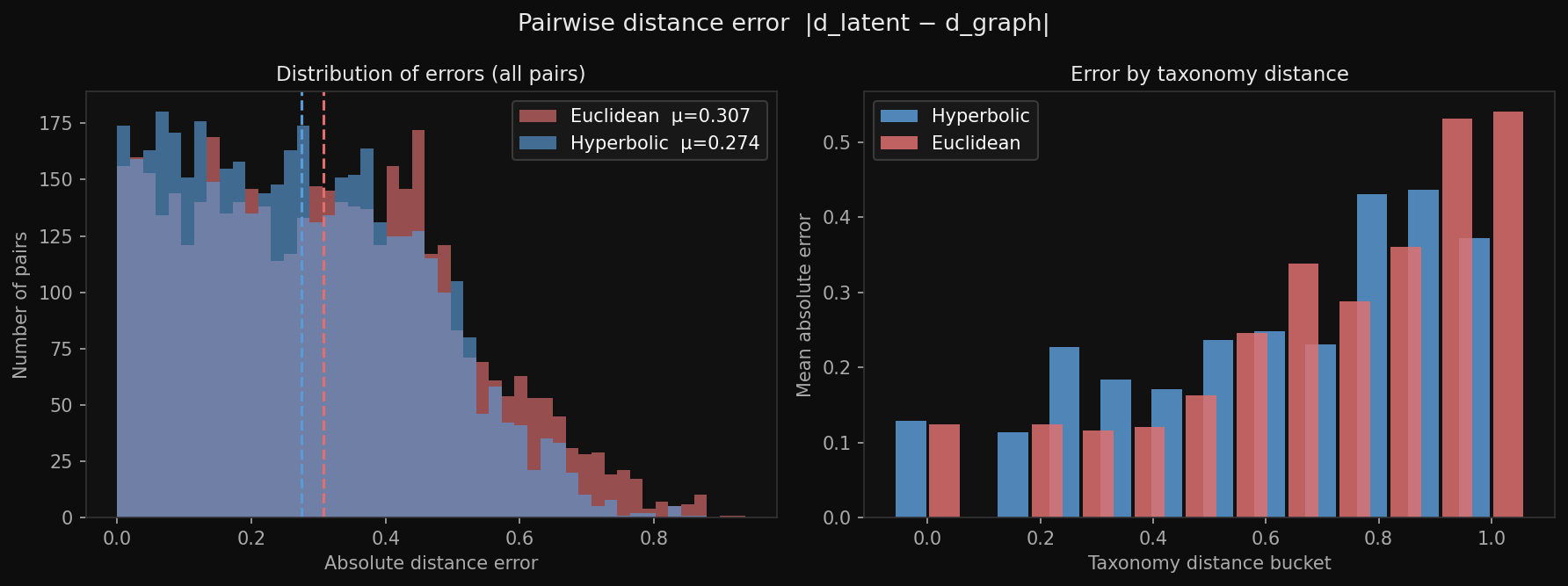
Left: distribution of |d_latent − d_graph| over all 4,371 pairs. Hyperbolic (blue) is shifted left — fewer large errors. Right: mean error by taxonomy distance bucket.
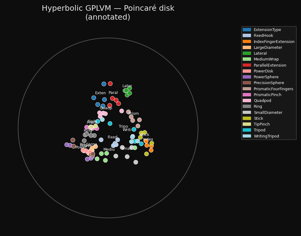
Final latent positions on the Poincaré disk, labelled by grasp class.
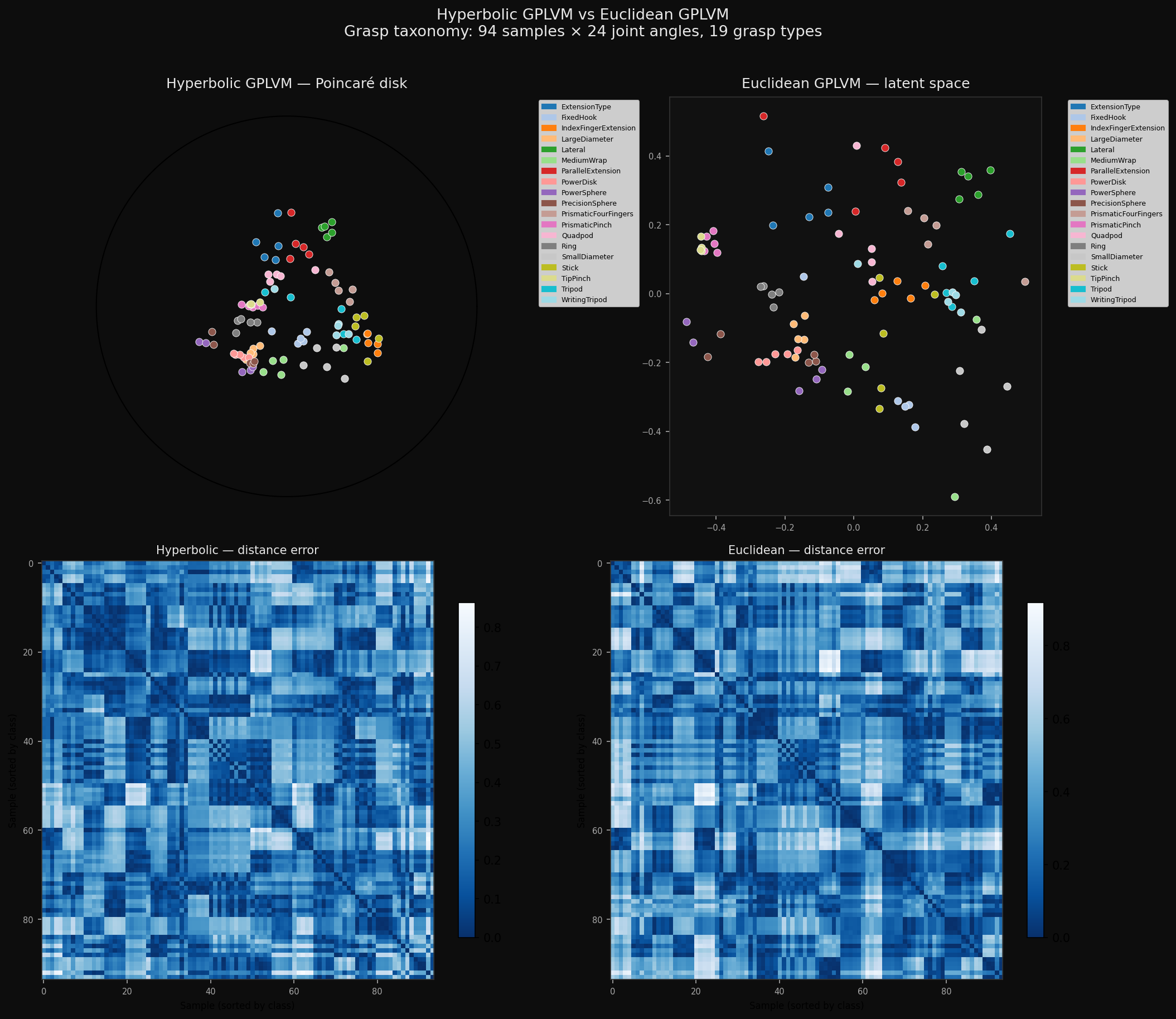
Hyperbolic vs Euclidean latent space + distance error heatmaps.
Everything written from scratch — no copy of the authors' code. 74 unit tests.
gphlvm/
├── lorentz.py    Lorentz geometry — inner products, geodesic distances,
│                 exp/log maps, Poincaré projection, wrapped-normal prior
├── kernels.py    Hyperbolic RBF kernel, stable Cholesky with adaptive jitter
├── gplvm.py      GP marginal likelihood, stress loss, full objectives
└── trainer.py    Two-phase training — geoopt RiemannianAdam on manifold
arccosh at the diagonal gives ~1.4×10⁻³ not zero due to floating-point
clamping — diagonal zeroed explicitly after the distance matrix computation.
Euclidean distance uses sqrt(d² + 1e-10) to avoid infinite gradients at
identical points. Cholesky uses adaptive jitter (1e-6 → 10.0) for early-training
near-singular kernel matrices.
git clone https://github.com/anshuman-dev/gphlvm-repro
cd gphlvm-repro
pip install torch numpy scipy networkx matplotlib geoopt pytest

python scripts/train.py --n-iter 1000 --stress-scale 5.0 --stress-warmup 300
python scripts/animate.py
python scripts/make_figures.py